HyLiTE algorithm
In this section, we discuss the main algorithm that HyLiTE is based on, along with some technical decisions and issues.
Preprocessing phase
Before entering the main HyLiTE algorithm, a number of steps are usually performed to move from the raw data to a form that can be used by HyLiTE main algorithm. During these steps, HyLiTE merely coordinates the calls to various external softwares.
The two programs that HyLiTE currently uses are bowtie2 and samtools.
The following figure details the operations performed during this preprocessing phase.
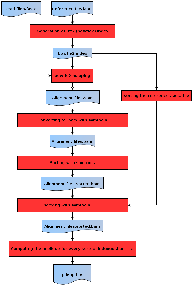
Flowchart of the preprocessing steps
Note
Until the pileup file is computed, each organism is treated independently.
Details about the input files can be found in the chapter 1. Basic considerations of the HyLiTE manual page.
The first step is to index the .fasta reference file (the file containing the gene models) using bowtie2-index. Then, each .fastq file (the files containing the reads) is mapped to the reference using bowtie2. Once alignment files in the .sam format have been obtained, each file undergoes a pipeline using samtools view, samtools sort and samtools index so as to make them usable by samtools mpileup. To function correctly, samtools index needs the reference .fasta file to be indexed using samtools faidx. Once all this has been completed, HyLiTE uses samtools mpileup to generate a unique .pileup file regrouping all the alignment information for every organism and biological replicate used in the study.
Because they rely on external software, these steps are not mandatory provided you already have the resulting files (for example, the .sam alignment file, or the .pileup file). Details about how to make HyLiTE skip these steps and how to run them yourself can be found in chapter 3. Using the different entry points of the HyLiTE manual.
Main algorithm
The following flowchart describes the main HyLiTE algorithm.
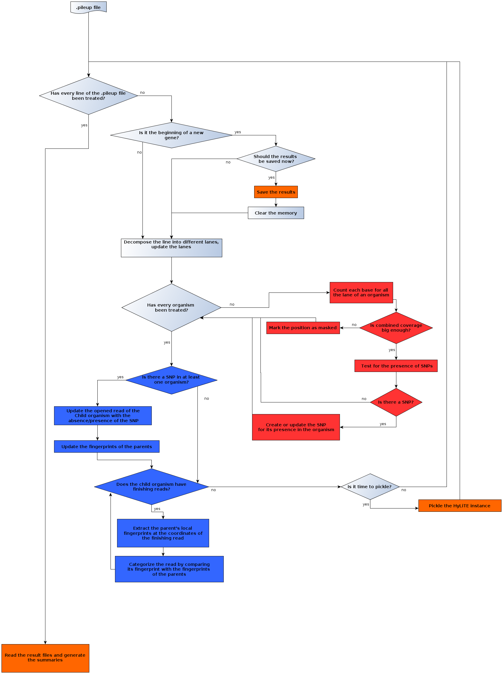
Flowchart of the main algorithm
The main algorithm consists of reading and ‘on-the-fly’ treating of the data contained in the .pileup file followed by a reporting proccess. The treatment of the information contained in the .pileup file relies heavily on the peculiarity of this format and can be divided into three parts:
Decomposing and interpreting a line of the .pileup file
Detecting SNPs (red in the figure)
Categorizing the reads (blue in the figure)
We can also distinguish the saving/writing steps, shown in orange on the flowchart.
1. Decomposing and interpreting a line of the .pileup file
As many concepts in HyLiTE rely on the .pileup structure, it is crucial to understand it in order to understand how HyLiTE works. Here is a simple example of a .pileup file with three organisms having only one sample each:
EfM3.000010.mRNA-1      1       A       2       ^K.^K,                          ::                      1       ^K.                            :                        1       ^K,             :
EfM3.000010.mRNA-1      2       T       6       .,^K.^K,^K,^I,                  ::9;97                  4       .^K.^K,^K,                     :9;9                     2       ,   ^I,         :7
EfM3.000010.mRNA-1      3       A       9       .,.,,,^K.^K,^K,                 ::7<:::;:               7       ..,,^K.^K,^K,                  :7<::;:                  2       ,,              ::
EfM3.000010.mRNA-1      4       T       15      .,C,,,.,,^K.^K.^K.^Ig^K,^K,     7<28999<;;9;0:<         11      .C,,.,,^K.^K.^Ig^K,             72899<;;90:             4       ,,^K.^K,        <9;<
EfM3.000010.mRNA-1      5       T       20      G,.,,,.,,...,,,^K.^K.^K.^K,^I,  2:9;<9:7:6::::;;9:;:    16      G.,,.,,..,,^K.^K.^K.^K,^I,      29;<:7:6:::;9:;:        4       ,,.,            :9:;
The first column is the ID of the current gene. The second column is the position in the gene. The third column is the reference base (i.e. the nuleotide at this position of this gene in the reference .fasta file). All other columns form different ‘lanes’.
Here, we call a group of three column a lane. For HyLiTE, a lane represents one sample from an organism. The three columns comprising a lane are, in order:
The coverage at that position (that is, the number of reads from this sample that map to this specific region of the reference gene )
The ‘pile’, a string representing the actual read content at that position
A string describing the local quality of the alignment (in PHRED format)
For instance, on the first line of the example, the first lane is:
2 ^K.^K, ::
The first and third columns of the lane are easily interpreted - here, the local coverage is 2 and the local PHRED quality of the base call for both reads is ‘:’ or 25. The second column, the pile, is however harder to understand.
Here are a few guidelines about the pile format:
the symbol . or , stand for a reference base match in the forward strand (.) or reverse strand (,)
mismatches are represented by the mismatching base, in uppercase for the forward strand, in lowercase for the reverse strand
the symbol ^ means that a read is beginning. It is followed by a symbol giving the PHRED quality of the entire read alignment
the symbol $ marks the end of a read
More details on the .pileup format can be found on the samtools page in the mpileup section.
So, in our first lane, the second column:
^K.^K,
actually represents two starting reads; the first comes from the forward strand, the second from the reverse strand.
Using this format, HyLiTE is able to obtain the base content for each individual read for any sample or organism at any given position.
2. Detecting SNPs
Once the content of every read (for each sample for each organism) mapping to a specific position on the model is known, HyLiTE can detect potential SNPs.
2.1 Error model
A single nucleotide mismatch from the gene on a read can have two origins: either it is an error introduced by the sequencing technology, or it is a SNP. In the case of haploid organisms, all the reads are expected to display the SNP. In the case of polyploid organisms however, the SNP could be present on one of the parental copies only and thus not all reads would display it.
To circumvent this problem, we use a very simple model for the insertion of errors by the sequencing technology. Let us consider a unique  , the probability that, at any position, an error is created on a read. So for every base in a read, there is a probability
  to find that this particular base is an error.
The distribution of errors along reads is not uniform. However, for a given coordinate on the gene (with the exception of gene extremities), the corresponding position along the reads aligning to this coordinate is quite uniformly distributed.
Furthermore, it is common practice to trim bases from the reads (in our case, we used SolexaQA) when their PHRED quality exceed a low threshold, thus guaranteeing a minimum level of quality for our entire read.
to find that this particular base is an error.
The distribution of errors along reads is not uniform. However, for a given coordinate on the gene (with the exception of gene extremities), the corresponding position along the reads aligning to this coordinate is quite uniformly distributed.
Furthermore, it is common practice to trim bases from the reads (in our case, we used SolexaQA) when their PHRED quality exceed a low threshold, thus guaranteeing a minimum level of quality for our entire read.
With these considerations in mind, the number of occurences of a specific error base (that is, a base that does not represent a real genotype) mapping at a specific position of the genome follows a binomial law with parameters  and
and  = number of reads (from a specific organism) mapping at that position (i.e. the local coverage).
It follows that if a mismatch does not follow such a binomial law, it can be considered as a SNP (note that the reverse is not necessarily true, and that we will address this problem later).
2.2 Parameters
To use the model described above, two parameters must be fixed:
- the probability of a base-specific error
 to test the hypothesis H0: ‘’the base is more frequent than if it followed a binomial law with parameters and , the coverage for this position’’
Note
This is a one-tailed test
has been estimated via a 19Gb .fastq file containing trimmed reads from a RNAseq experiment generated by Illumina sequencing. The total e has been estimated as 0.02. Thus we use  .
.
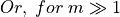
As testing for the presence of SNP is made for every position in the gene for every organism, a very large number of independant tests is recquired and, thus, cannot be used as is and must be corrected for multiple testing.
Because we do not know anything other than the number if test  is
is  and for the sake of simplicity, we use the Rough False Discovery Rate (RFDR) to correct our . Thus
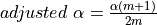 ,
,
 ,
,
So for a global risk of 0.01 we have to choose  . However, empirical practice has lead us to reduce the parameter to a more conservative value of 0.001.
2.3 Minimum coverage and MDER
The second parameter of the binomial law allowing us to distinguish between SNPs and errors is the local coverage.
The binomial law is a discrete law, and it is known that if  is too small in relation to , then the predicted value does not reflect .
Our estimated is quite small ( ) and fixed while our value for changes (this is the local coverage). So we have to determine a limit for under which the values predicted by the binomial law are not satisfying.
For example, with a coverage of 2, the expected number of occurences is 0. That would mean that an error on a read at that position would automatically be detected as a SNP which is undesirable.
As a rule, we state that any expected value is, at a minimum, 2.
For haploid organisms, only one genotype is expected and detected. Given the minimum expectancy of 2, a coverage of 3 reads is sufficient to detect the true genotype with high accuracy. Under a coverage of three, the position is marked as MASKED, which means that it will not be used for parental categorization of the hybrid’s read.
For polyploid organisms, multiple genotypes can be expected (in fact, the categorization relies on this). Furthermore, RNAseq data do not offer a guarantee of equal representation of each genotype (i.e. the different parental copies of a gene will not necessarily have the same expression). Thus we consider the ratio of expression between the least expressed genotype and the sum of the other genotypes (if a gene copy is expressed 10 times when the other is expressed only once, the expression ratio is  ).
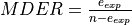
This allows us to define the minimum detected expression ratio (MDER) as the limit under which the least represented genotype would be detected as an error. So, for , and (the coverage) fixed, the MDER corresponds to the expected number of occurences of a specific error (
).
This allows us to define the minimum detected expression ratio (MDER) as the limit under which the least represented genotype would be detected as an error. So, for , and (the coverage) fixed, the MDER corresponds to the expected number of occurences of a specific error ( ) divided by
  .
.
The following figure represents the evolution of the MDER as the coverage increase.
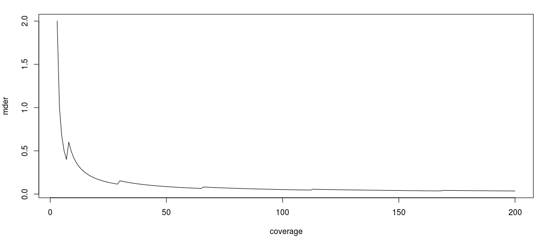
Please note that the jagged effect of the curve is due to the discrete character of the binomial law.
Any value above 0.5 does not make any biological sense. Otherwise, the MDER shows a tendency to decrease as the coverage increases (its limit when the coverage is infinite being ). This basically means that the better the coverage, the better you will be able to detect a large difference in expression level between different parental copies of a gene.
The following figure shows an enlargment of the preceeding figure.
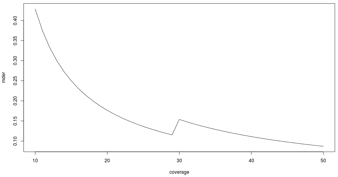
Here we can clearly see that for a coverage of 20, the MDER is 0.18 (exactly,  ) and it does not increase as the coverage increases. We suggest that this value should serve as a minimum coverage for the polyploid species. This means that, independently of the coverage, a MDER greater than or equal to (i.e. a Minor Allele Frequency greater than or equal to 0.15) will always be detected if the coverage is greater than or equal to 20.
If the coverage is lower than 20, the position will be marked as MASKED.
2.4 The algorithm
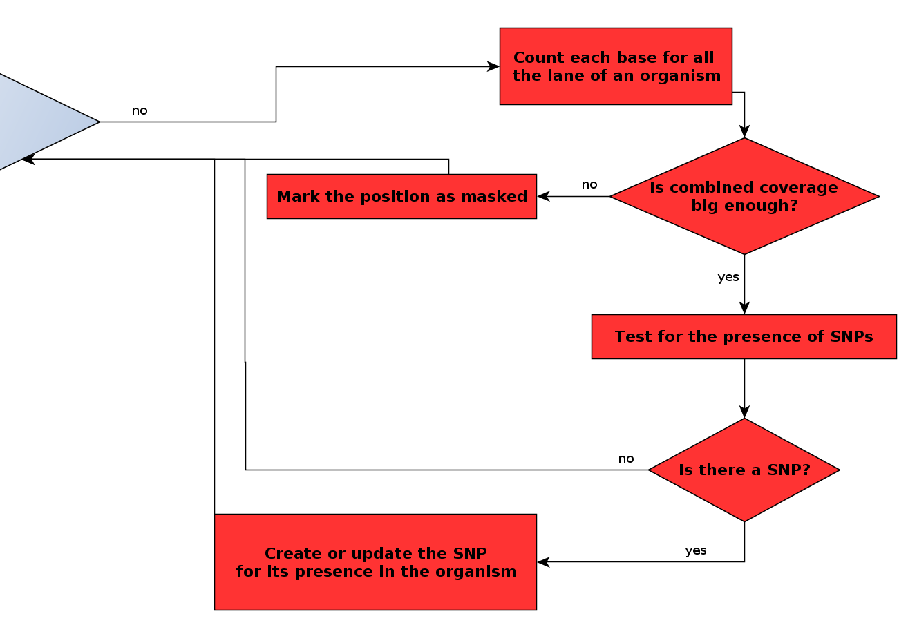
Flowchart of the main algorithm - detail of the SNP detection loop
Now that we have laid out the theory behind SNP detection, describing the algorithm is relatively easy. At a given position, for a given organism:
First, HyLiTE temporarily agregates the different lanes (biological replicates) of an organism. Thus, the coverage becomes the sum of the coverage for the different lanes
Then, HyLiTE counts and compares every genotype to its expected count if it were an error.
The n best selected genotypes are considered valid (where n is the ploidy of the organism)
Each valid genotype different from the reference is considered as a SNP present in the organism.
Note
At this stage, presence of a SNP in an organism means that the new base is present in at least a few of the reads.
The artificial increase in the coverage during the first step provides a way to avoid masking positions and decreasing MDER
For example, at a given position with a reference of A, a diploid hybrid with two lanes displays:
lane1: A:14  T:1  G:54  C:2
lane2: A:5   T:0  G:14  C:0
after aggregation of the two lanes, the counts are:
A:19 T:1 G:68 C:2
for a total coverage of 90 which is greater than the minimum coverage for polyploids, 20. For such coverage, the threshold for valid genotype detection is 5 (according to the binomial law). This means that after comparision, only two possible genotypes remains: A and G. As the organism is diploid, at most two possible genotypes can be present at the same position, which does not eliminate any possible genotype here. A being the reference, we conclude that there is a SNP at this position with an alternative allele G and that it is present in the hybrid organism.
3. Categorizing reads
One of the main features of HyLiTE is the capacity to determine the parental origin of the hybrid’s reads. The next figure details how this is done.
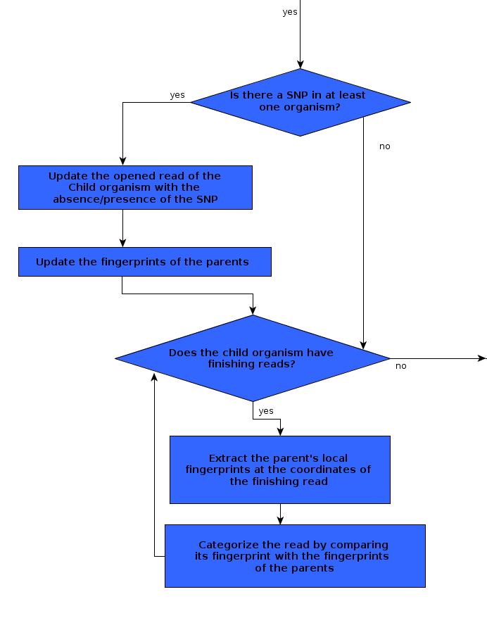
Flowchart of the main algorithm - detail of the steps leading to categorization
3.1 Fingerprints
By fingerprints, we refer to the sequence of the SNPs present, absent, or masked because of bad coverage, at specific positions in a gene.
We distinguish two types of fingerprint:
Parent fingerprint: where information about absence, presence and masking for the parent are stored, gene-by-gene.
Child fingerprint: each of the hybrid reads has its own fingerprint, referencing absence or presence of every SNP on that specific read.
Note
Masking is never referenced on read fingerprints as this would mean that the read does not exist at that position.
3.2 Fingerprints and read tagging for diploid parents
When a parent is diploid, it usually possesses two fingerprints at each SNP position in order to accommodate possible heterozygosity. Accounting for this heterozygosity is achieved locally through read tagging.
Read tags have three possible values: unassigned, gene copy 0, and gene copy 1. Each parent read begins with an unassigned tag. Whenever a heterozygous position is detected in the parent, HyLiTE first looks for reads with an assigned tag. If there is no read with a tag assigned (as it is the case at the start of each gene), gene copy 0 or 1 is arbitrarily assigned to the allele and each read is tagged according to this classification. However, if some reads are already tagged (i.e., they have already been assigned to a gene copy), HyLiTE determines which allele coincides with which tag and then propagates those tags to all reads bearing those alleles.
In this way, when the fingerprints of the parents are updated, any alleles detected are ordered by gene copy number in order to stay coherent and produce two well separated fingerprints.
3.3 Algorithm
Remember that HyLiTE detects SNPs at a given position for every organism sequentially. This means that when HyLiTE proceeds to a new position, all the SNPs located before that new position have already been detected. This is very interesting as it means that as soon as one of the hybrid’s reads finishes (at the far end of the read, in terms of model coordinates), all the SNPs that it could have presented have already been detected and referenced in every organism as well as itself. Thus, HyLiTE can directly proceed with its categorization.
To understand the categorization for an organism, remember that we store the presence of every SNP as well as its absence (and masking). So information about every detected SNP is accessible for the desired region (that is, between the start and the stop of the finished read). Thus, after the removal of MASKED SNPs (that is, SNPs where at least one organism presents bad coverage), we can model our read by a list of 0s and 1s, where 0 indicates the absence of a SNP and 1 its presence. We can do the same for each parent.
Then, categorization comes down to a series of comparisons between the parent and the child fingerprints. That is, comparison between lists of booleans.
Eliminate any child-specific SNP for the various fingerprints. If any SNP is eliminated, set an N flag meaning that there is at least one non ancestral SNP on this read.
Perform a bitwise XNOR operation between the child fingerprint and the fingerprint of each parent.
If the result of any of these XNOR operations is a list composed only of ones, the read is considered as coming from this parent (because the fingerprints match) and the categorization is done
Note
If multiple parents exhibit a perfect match, then the read category explicitly indicates that it could come from one or another parent.
If no perfect match is found, recursively try to cross parents together until a perfect match is found.
Note
The ‘crossing’ operation is merely an OR operation between parent XNOR results
Scenarios implying crossing between fewer parents are preferred
3.4 Examples
Simple example
Let us consider a read r of a hybrid from two parents, P1 and P2. r goes from position 35 to position 124 on gene1. Here is the position of SNPs in that region, along with absence/presence/masking information for r (the read), P1 and P2:
position    r     P1    P2
40          1     1     -1
52          1     0     0
65          1     1     1
96          1     0     1
113         1     1     1
Where 1 signifies the presence of the SNP, 0 signifies the absence of the SNP and -1 signifies a masked SNP (bad coverage for that organism at that position).
The first step is to eliminate the MASKED SNP at position 40. Then, the fingerprints of each organism are obtained as follows:
r: 1111 P1: 0101 P2: 0111
1. Child-specific SNPs are removed. For the first SNP, none of the parent displays a presence while r do: this is a child-specific SNP. Thus a flag N is raised. The fingerprints are now:
r: 111 P1: 101 P2: 111
2. A XNOR (here noted EQ) operation is performed between r fingerprints and each parent’s fingerprints:
r EQ P1: 101
r EQ P2: 111
In the previous step, r EQ P2 yielded a fully positive result, while r EQ P1 did not. We can then conclude that P2 is the likely parental origin of the read r
Thus the category assigned to r will be (P2)+N (remember that we raised the N flag indicating a child-specific SNP)
Note
The use of parentheses seems redundant in these simple cases. It becomes crucial when dealing with more than two parents and several origin scenarios.
Complex example
Let us now consider a read r from a hybrid of three parents, P1, P2 and P3. All preliminary steps, including removal of MASKED and child-specific SNPs leads to the fingerprints:
P1: 1011    P2: 1110    P3: 0001
            r: 1101
The XNOR operations yield:
r EQ P1: 1001
r EQ P2: 1100
r EQ P3: 0011
None of the results is comprised of 1s only, so r is probably a chimeric read (the result of a recombination between two or more parental copies). First, we test for a biparental crossover scenario by performing a bitwise OR operation between any combination of two of the results yielded by the previous XNOR operation. Here:
P1 + P2: 1101
P1 + P3: 1011
P2 + P3: 1111
Note
Here, “P1 + P2” actually means a bitwise “(r EQ P1)OR(r EQ P2)”.
One result yields only 1s and is therefore a suitable category for r: (P2+P3).
4. Saving processes
There are three points in the algorithm when HyLiTE writes out files.
4.1 Pickling
This operation is performed during the reading of the .pileup file, every 50 genes by default. It allows any crashed HyLiTE session to be restored. It generates a .pickle file with the name of the HyLiTE analysis as a prefix.
Note
How to restore a crashed HyLiTE instance and change the rate of the pickling is treated in Restoring a crashed HyLiTE run of the HyLiTE manual page.
4.2 Saving results
By default, this operation is performed as soon as a gene is finished. It comes from two factors:
genes are independant for SNP detection and categorization of reads
the cost in memory to store all gene information at the same time is enormous
Note
This memory cost also has an effect on the time cost of the software: the time required for pickling increases exponentially with the number of genes held in memory.
So, each time a gene finishes (i.e, all its positions have had their SNPs detected, all its reads have been categorized), HyLiTE appends the SNP and read information to the simple results files (you can learn more about these files in HyLiTE output formats) and this information then is cleaned from the memory.
4.3 Writing summaries
This is the last step of a HyLiTE analysis. Once the .pileup file have been read and treated, HyLiTE goes through the results files and creates additionnal results files called ‘summaries’. These summaries group the information by gene rather than by individual SNP or read (you can learn more about these files in HyLiTE output formats).